Continuing the documentation of a self-study exercise of working through the Robot Mapping course offered by Autonomous Intelligent Systems lab at the University of Freiburg.
- Autonomous Intelligent Systems #1: Robot Mapping
- Autonomous Intelligent Systems #2: Robot Mapping
- Autonomous Intelligent Systems #3: Robot Mapping
Note: sheet 2 was skipped as it was just an example application of bayes theorem.
Before attempting the problem set (sheets) complete the slides + recording.
Exercise 1.a: Describe briefly the two main steps of the Bayes filter in your own words.
The 2 main steps consists of a predict step and an update step. The predict step propagates a belief of the state and error covariance through a system model to obtain an a priori estimate for the next time step. [1] The update step takes the a priori estimate and corrects/updates with a measurement, incorporating new information to obtain the a posteriori estimate.
Exercise 1.b: Describe briefly the meaning of the following probability density functions.
- \(p(x_t | u_t, x_{t-1})\) → distribution of the state at time,\(t\), given a control action applied from a state at time \(t-1\).
- \(p(z_t | x_t)\) → distribution of a given measurement at time \(t\), given the state at time \(t\).
- \(bel(x_t)\) → a priori belief, and the current estimate of the distribution of the state at time \(t\).
Exercise 1.c: Specify the distributions that corresponds to the above mentioned 3 terms in the EKF.
- \(p(x_t | u_t, x_{t-1})\) → The mean is \(g(\mu_t, u_{t-1})\), while the covariance is the matrix Q representing the process noise.
- \(p(z_t | x_t)\) → The mean is \(h(\mu_t)\), while the covariance is the matrix R representing the measurement noise.
- \(bel(x_t)\) → \(\mu_t\) the state estimate at previous time step before putting through system model and covariance is \(\Sigma_t\).
Exercise 1.d: Explain in a few sentences all of the components of the EKF algorithm.
- \(\mu_t\) → state estimate at time \(t\), (n,1)
- \(\Sigma_t\) → covariance matrix at time \(t\), (n,n)
- \(\bar{\mu_t}\) → state estimate propagated through time using the process model., (n,1)
- \(\bar{\Sigma_t}\) → covariance matrix at time \(t\) updated with Jacobian, G, and process noise, Q. (n,n)
- \(g\) → function to update state space based on some motion/process/system model., (n,1)
- \(G_t^x \) → Jacobian of the motion matrix. (n,n)
- \(R_t\) → measurement noise, (m,m)
- \(h\) → measurement function, (m,1)
- \(H_t^x\) → Jacobian of h, (n,m)
- \(Q_t\) → process noise, (n,n)
- \(K_t\) → Kalman gain
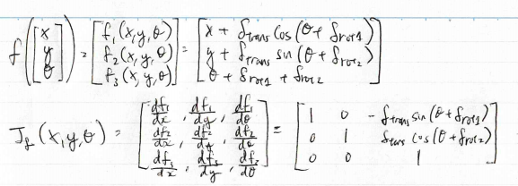
Exercise 2.a: Derive the Jacobian matrix \(G_t^x \) of the noise-free motion function \(g\) with respect to the pose of the robot. Use the odometry motion model as in exercise sheet 1.
Apologies for the sloppy hand writing. Will port to latex at some point
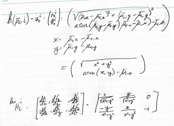
Exercise 2.b: Derive the Jacobian matrix \(H_t^i\) of the noise-free sensor function \(h\) corresponding to the \(i^{th}\) landmark.