Update: 2020/Feb/3rd Hi thanks for stopping by. Why not checkout https://www.korabo.io. The app allows you to set percentage share with collaborators and generate different types of entry points to a checkout like the shield below.

+++++++

Working through some classic CV algorithms to refresh the memory, I am constantly reminded of the ingenuity of the algorithms and the researchers behind the work. In this memory refresh (post), I plan to work through the algorithm related to Laplacian Pyramids and its application to image composition, or equivalently blending stated differently.

The objective of the procedure is to produce a seamless image, given two images as inputs, or as Burt and Adelson stated,

How can the two surfaces be gently distorted so that they can be joined together with a smooth seam?

The location of the blend is variable and is case dependent. The mask, controls the location and degree of the blend, and the set of possible masks that one can contrive is large.

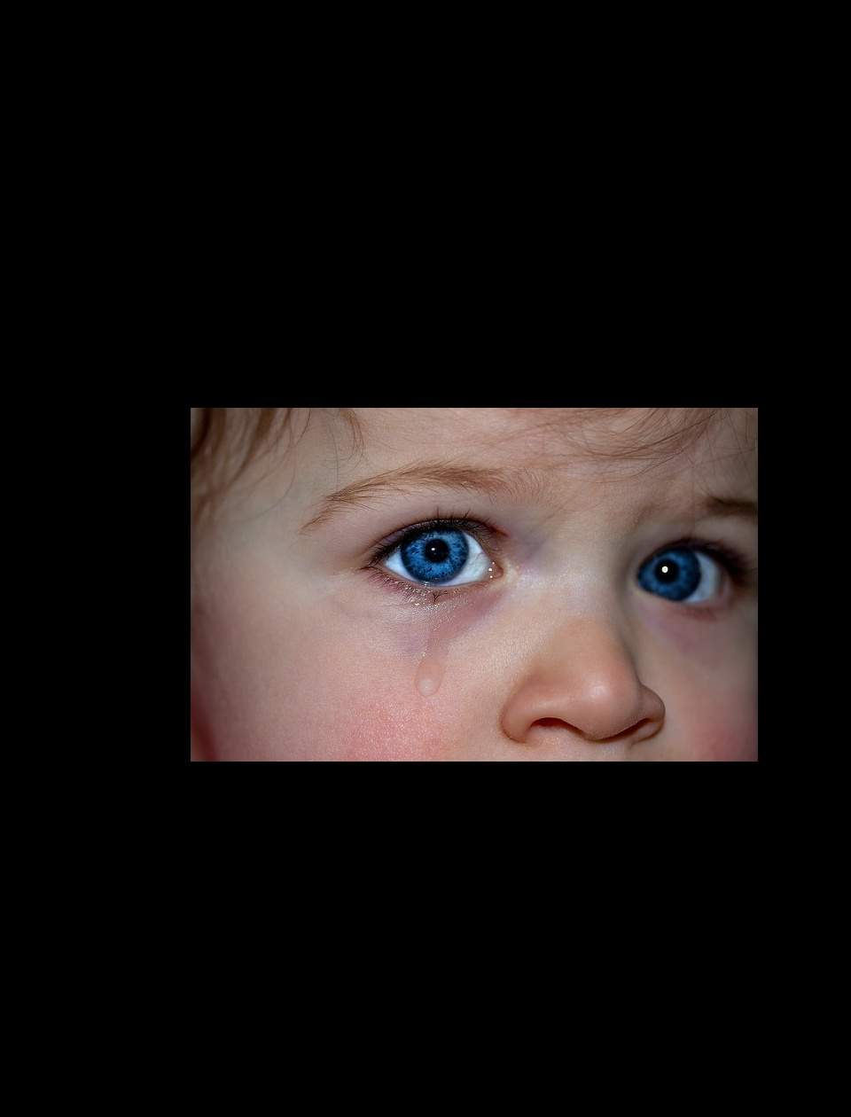
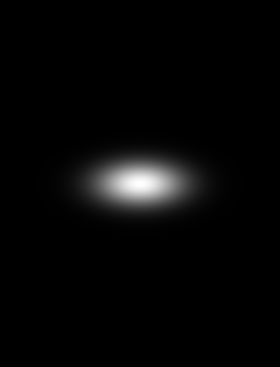
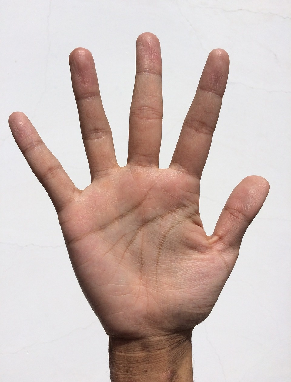
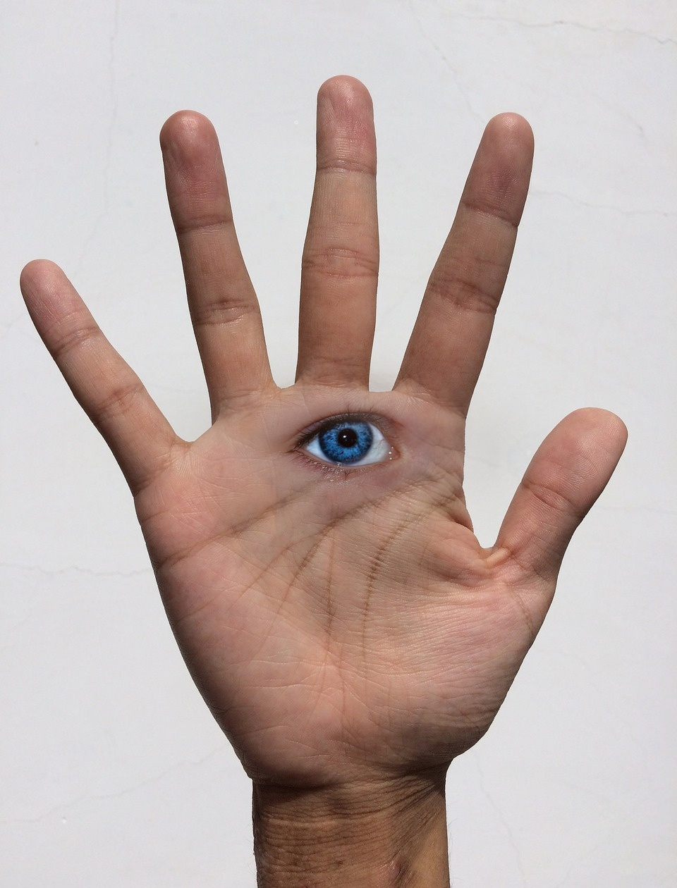
Taking two images A(left), and B(right), and a mask, M(center), presented above, we can blend the images utilizing Laplacian pyramids to construct a blend that results in the following image. There is scope for automation, but for this exercise, the location of eye was manually engineered to “work”.

In the following section I will introduce the procedure that underlies the Laplacian Pyramid, and discuss the relevance and importance of engineering an appropriate mask.

Constructing the Laplacian Pyramid

The details of the algorithm can be found in the publications by Burt and Adelson [1,2], thus I will skimp on the details, and recommend the reader to work through the paper. A top level overview of the algorithm is as follows:

• Construct the gaussian pyramids.
• Construct the laplacian pyramids.
• Create the blended pyramids.
• Collapse the blended pyramids to reconstruct the original image exactly.

To start, we need to determine the number of layers of the pyramid, which can be done given the dimensions of the original image, and kernel, and satisfying the following equations. \[C = M_c2^{N}+1\] \[R = M_r2^N + 1\] where C is the columns size, R is the row size, \(M_c\) and \(M_r\) are equivalent to \(\frac{1}{2}\) (kernel size - 1), and N being the number of layers. Thus, if we have the dimensions of the image, and kernel, we can calculate the number of layers: \[N = floor(\log_2(\frac{R-1}{M_r})\]

Once we have determined the number layers we can construct the gaussian pyramid, using the $reduce()$ function to convolve and then downsample over the given number of layers. The open source OpenCV library[3] has the pyrDown() function which uses a \(5\times5\) kernel shown below, to convolve, and downsamples by rejecting the even number rows and columns at each successive layer.

The algorithm itself is rather trivial to implement, using the filter2D() function found in the OpenCV library, which handles the padding and convolution step.

A personal rendition of the reduce function:

def mypyrDown(image, kernel):
    image = image.astype(dtype=np.float)
    dst = cv2.filter2D(image, -1, kernel, borderType=cv2.BORDER_REFLECT)
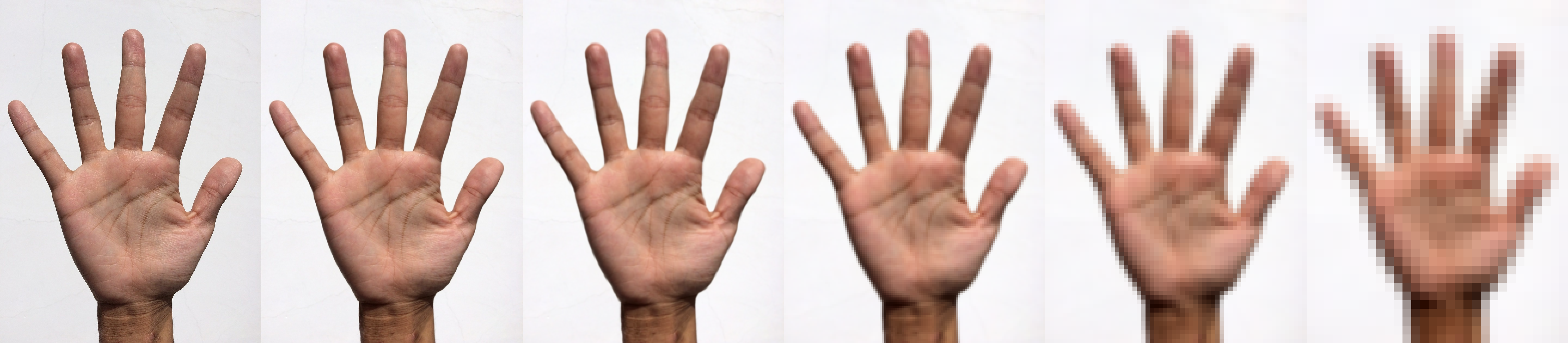
    return dst[::2, ::2].astype(dtype=np.float64)

This should leave us with N - 1 downsampled images, with the original image used as the base of the “pyramid”. The effect of the reduce operation is in effect applying a low-pass filter. The convolve step is an averaging operation, which takes pixels in the neighborhood and applies a linear transformation. This basically has the effect of dispersing the local per pixel information. The downsample, reduces redundancy and correlation of the pixels. This works on the idea that neighbor pixels are correlated. The following image is the gaussian pyramid, with each layer scaled to match original. We can see clearly how the fine features are removed and we are left with a rather course representation in the final layer.

Construction of the Laplacian Pyramid involves upsampling, padding then convolving with the same kernel used in the downsample. pyrUp() can be used for this. The construction itself is recursively applying pyrUp() to a layer in the Gaussian Pyramid and subtracting from the next layer. The procedure starts with the smallest layer. At each step, the procedure effectively is isolating the error between two images, the original image and the averaged image, with the error interpreted as the high frequency information lost in the convolution and downsample step. Again, the implementation is relatively trivial, and really highlights the ingenuity of the designers. Simple yet powerful.

#The code was written for clarity over efficiency
def mypyrUp(image, kernel):
    r,c = image.shape
    uns = np.zeros((r*2,c*2))
    uns[::2,::2] = image
    dst = cv2.filter2D(uns, -1, kernel, borderType=cv2.BORDER_REFLECT)
    return dst.astype(dtype=np.float64)*4

def mygaussPyramid(image, levels):
    lst = [image.astype(dtype=np.float64)]
    for _ in range(levels):
        image = reduce_layer(image)
        lst.append(image)
    return lst

def mylaplacianPyramid(gaussPyr)
    retlst = []
    layers = len(gaussPyr)
    count = 0
    for i in range(layers):
        if i < layers-1:
            r,c = gaussPyr[i].shape
            retlst.append(gaussPyr[i] - expand_layer(gaussPyr[i+1])[:r,:c])
    retlst.append(gaussPyr[-1])
    return retlst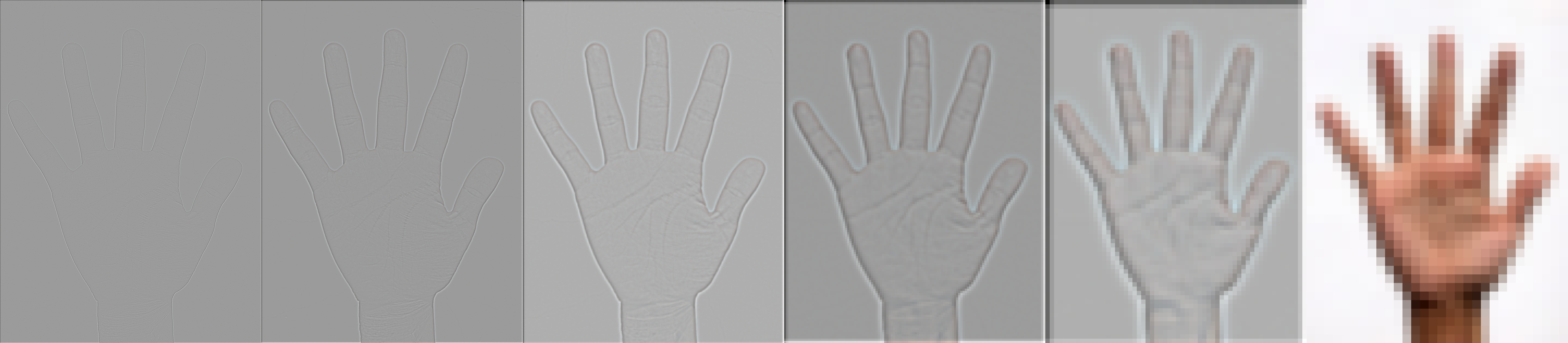

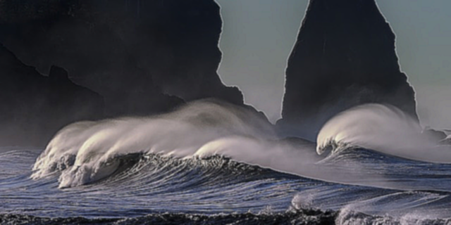
Just to expand on the concept of the effect of a low pass filter, we can consider the unsharp masking method used to sharpen images. \[g_{sharp} = f + \gamma(f-h_{blur}\star f)\] The process extracts the difference, error, between an image, and the average image, and adds back some proportion of this difference. The idea is that the error represents areas of high intensity, and accentuates the given area by doubling(not literally) down. The following images displays the results of the unsharp mask operation. [Original, Blurred, Sharpened]

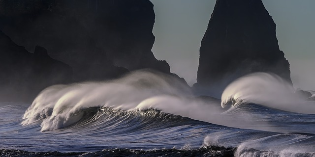
See the associated code for completeness.

gbeach = cv2.GaussianBlur(beach, (5,5), 1)
sharp =cv2.addWeighted(beach, 1.5, gbeach, -0.5, 0, beach)

Will cover blending and collapsing in the next post, followed by a brief discussion on masks…

(All mistakes are mine, any corrections appreciated.)

References:

1. Burt, Peter J and Adelson, Edward H. A Multiresolution Spline with Application to Image Mosiacs
2. Burt, Peter J and Adelson, Edward H. The Laplacian Pyramid as a Compact Image Code