I came across a video by Martin Gorner, which can viewed here. The presentation provides a top level, yet self contained overview of deep learning and tensorflow.
I found his presentation of the LSTM cell informative, in particular, the way he chose to present the concept had impact on my learning process.
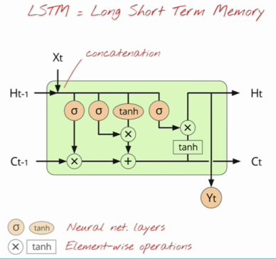
The specific segment on the LSTM cell contained a walk through of the components of the cell, stepping through each gate.

- Concatenate: \(X= X_t | H_{t-1}\)
- Forget gate: \(f = \sigma(XW_f + b_f)\)
- Update gate: \(u = \sigma(XW_u + b_u)\)
- Result gate: \(r = \sigma(XW_r + b_r)\)
- Input: \(X’ = \tanh(XW_c + b_c)\)
- new C: \(C_t = f * C_{t-1}+u*X’\)
- new H: \(H_t = r * tanh(C_t) \)
- Output: \(Y_t = softmax(H_tW +b)\)
- The concatenate step takes \(X_t\) and concatenates with \(H_{t-1}\) resulting in a vector with dimensions \(p+n\). As the other gates are working in dimension \(n\), we need a transformation that maps \(\mathbf{R}^{p+n} \rightarrow \mathbf{R}^{n}\), thus need to apply \(W_i\) where \(i\in {f,u,r,c}\).
- \(C_t\) is the result of applying the forget gate, \(f\), which regulates what is forgotten and what remains. The result of applying \(f\), element wise, is summed with the update gate, \(u\), applied to \(X’\) elementwise. The internal state of the cell is updated in this manner.
- Note that the sigmoid non-linearity, \(\sigma\), applied in the forget, update, and result gate, squashes the result between 0 and 1, thus acting as a discount factor.
- Another point raised, is the reason we apply the \(\tanh\), non-linear function. Note that \(C_t\) is the sum of two positive operands, thus easily can result in divergence. By applying \(\tanh\) the result is squeezed between -1 and 1, thus helping to mitigate the risk of divergence.
Keep in mind that this is one possible structure for an LSTM cell…the possibilities of combinations are limitless though, in contrast, the differentiation on performance as a result of cell structure appears limited.