
Update: 2020/1/22
If you find this article at all helpful, please consider a supportive contribution.

Overview
In the paper, “DEX: Deep EXpectation of apparent age from a single image”, the authors were able to display remarkable results in classifying the age of an individual based on a given single image. The results were obtained using an ensemble of convolutional neural networks. The model design process consisted of starting with a VGG-16 architecture pre-trained on image-net which was fine-tuned on the IMDB-WIKI data set. This is followed by training on the ChaLearn LAP data set. The data set is split in 20 sub data sets. Though a random process was followed in the paper the authors were careful in maintaining the distribution of the original data set for each subset. This results in 20 different trained models where the final prediction used was the average of the ensemble of 20 networks trained. See the paper for the exact details, as this is just a high level summary.
The data set is large enough to the extent that in memory management is non-trivial. The IMDB data set is 269GB while the face-crop version is 7GB. Trying to pre-process this data set, let alone train, is beyond the scope/capacity of an individual with limited resources. The challenge for this particular exercise is to see the results of using a small subset of the original data and using a lower capacity architecture.
For some perspective, training on the architecture proposed by the authors took 5 days to train on the entire IMDB + WIKI data set.
source: https://github.com/surfertas/deep_learning/tree/master/projects
UPDATES: Apr/07/2018: IMDB-WIKI: notes on refactoring data preprocess pipeline
Data: faces only (7GB)
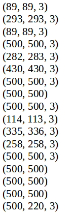
The data is relatively “raw” as the provided data (at least the face-crop version) was inconsistent in dimensions, and color channels. The authors suggest this was the case as the data was collected using a web-crawler. Just to give an example, the dimensions of a few samples from the training set are listed below. We can see that some are colored and some are gray scale, while the sizes are not consistent. The formatting steps taken here were to convert all images to gray scale, and resize images to dimensions of \(128\times128\). A simple python script can handle this processing.
That was just handling the images. Now we need the labels, which again was not easily obtained. The meta data is stored separately and unfortunately in a .mat file. (Yes, matlab). The meta information stored is as follows: dob: date of birth (Matlab serial date number)
- photo_taken: year when the photo was taken
- full_path: path to file
- gender: 0 for female and 1 for male, NaN if unknown
- name: name of the celebrity
- face_location: location of the face. To crop the face in Matlab run img(face_location(2):face_location(4),face_location(1):face_location(3),:))
- face_score: detector score (the higher the better). Inf implies that no face was found in the image and the face_location then just returns the entire image
- second_face_score: detector score of the face with the second highest score. This is useful to ignore images with more than one face. second_face_score is NaN if no second face was detected.
- celeb_names (IMDB only): list of all celebrity names
- celeb_id (IMDB only): index of celebrity name
The label that we require for training is the age parameter, which is not
stored as meta information, and requires some calculation. The age value can be
obtained by taking the
photo_taken and subtracting dob, the date of birth. Sounds easy? No…as the
dob is stored as a Matlab serial number.
Luckily we can use the scipy.io.loadmat to load the .mat file to a python
consumable (kind of) format. We can access the dob by some proper indexing,
and convert the Matlab serial number to a usable format by using
datetime.date.fromordinal( serial_number ).year. Ok, so now we have the dates
in a consistent format thus extracting the age is now trivial.
Now the inputs, \(128\times128\) gray scale images, and labels, estimated age, can be
packaged together and dumped to a pickle file. The script can be found
here.
The script allows the user to specify the size of the training set, by setting
the parameter --partial.
Training
Now we are ready for training. Keep in mind, we are using only a subset of the data, and using an experimental self-designed model that has a much smaller capacity. Further, the model was not pre-trained on Imagenet thus we need to take steps to adjust accordingly to increase the odds of success.
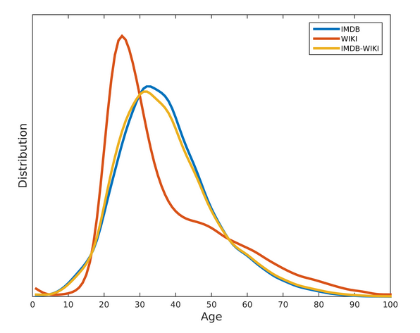
The original paper uses \(101\) age classes, which was appropriate for the data set size and learning architecture used. As we are only using a subset of the data and a very simple model, the number of possible classes was reduced and set to 4, {Young, Middle, Old, Very Old}, with the bucketing defined by Young \((30yrs < age)\), Middle \((30 \leq age < 45)\), Old \((45 \leq age < 60)\), and Very Old \((60 \leq age)\). The distribution of the data gets concentrated around \(30-60\), see the below image for the distribution of the ages for each data set. [2] The images were preprocessed using ZCA Whitening.
The model used for this exercise is shown below (the Chainer framework was used for implementation). Basically the model consisted of 3 convolution layers, with ReLU activition, batch normalization, max-pooling, and dropouts applied, basically any form of regularization was used that might help in reducing training time, and risk of overfitting, and as a result increase learning ability to compensate for the lack of data and capacity of the model.
class CNN(chainer.Chain):

    def __init__(self, n_out):
        super(CNN, self).__init__(
            conv1=L.Convolution2D(1, 32, ksize=3, stride=2, pad=1),
            bn1=L.BatchNormalization(32),
            conv2=L.Convolution2D(32, 64, ksize=3, stride=2, pad=1),
            bn2=L.BatchNormalization(64),
            fc3=L.Linear(4096, 625),
            fc4=L.Linear(625, n_out)
        )

    def __call__(self, x):
        h = F.relu(self.bn1(self.conv1(x)))
        h = F.max_pooling_2d(h, ksize=2, stride=2, pad=0)
        h = F.dropout(h, ratio=0.3, train=True)
        h = F.relu(self.bn2(self.conv2(h)))
        h = F.max_pooling_2d(h, ksize=2, stride=2, pad=0)
        h = F.dropout(h, ratio=0.3, train=True)
        h = F.dropout(F.relu(self.fc3(h)), ratio=0.3, train=True)
        return self.fc4(h)
Results
The first 10,000 images were used with the distribution of data is as follows:
- YOUNG: 0.1381
- MIDDLE: 0.4439
- OLD: 0.3386
- VERY OLD: 0.0794
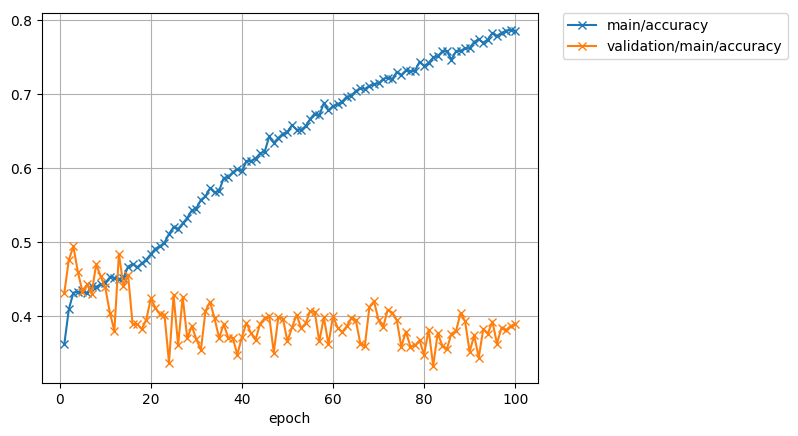
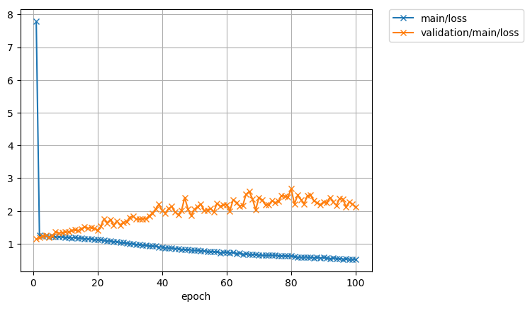
Well as one would expect, the results are quite poor on this first pass. The model used fitted(over) to the dataset well, while the test accuracy shows really no improvement and seemingly cant do much better than random guessing. Realistically this was fully expected as the capacity of the model, and size of the data set was extremely constrained. Lack of pre-training on image-net is a consideration that likely impacted as well. The exercise was really just an exercise, and a good lesson about how data is not always in consumable form, and the importance of the general infrastructure necessary to properly train and learn on data of any meaningful size.
That said, it is likely too early to form a conclusion. Will make further attempts with different architectures.
References
[1] Rothe, R., Radu, T., Van Gool, L. DEX: Deep EXpectation of apparent age from a single image. [2] https://data.vision.ee.ethz.ch/cvl/rrothe/imdb-wiki/