
Previous Posts:
- Actor-Critic and Policy Gradient Methods #1
- Actor-Critic and Policy Gradient Methods #2
- Actor-Critic and Policy Gradient Methods #3
- Actor-Critic and Policy Gradient Methods #4
Having developed a decent understanding of the policy gradient method in the derivation of the gradient of the objective function, \(\nabla J(\theta)\), we can use the gradient ascent algorithm to optimize an objective function, parameterized by \(\theta\), with the \(J(\theta)\) representing the quality of a policy.
Before we step ahead to the Actor-Critic algorithm, best to introduce the REINFORCE algorithm, which only has an actor, and uses PGM to optimize the objective function. The lack of the critic, which has variance reducing properties, exposes the algorithm to high variance. The psuedo-code is taken from D.Silvers lectures on Policy Gradient Methods.
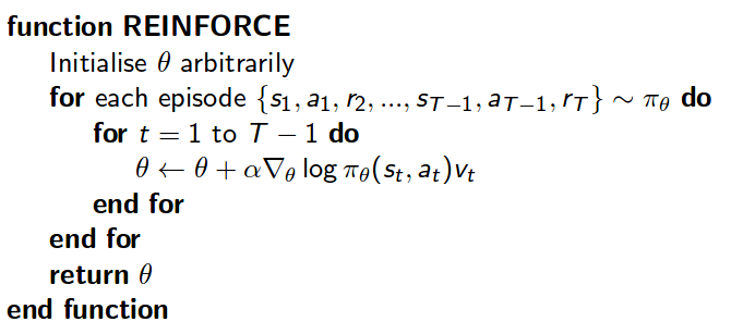
Lets consider the Policy Gradient Theorem.
\[\nabla_{\theta}J(\theta) = E_{\pi_{\theta}}[\nabla_{\theta}\log\pi_{\theta}(s,a)Q^{\pi_{\theta}}(s,a)]\]\(Q^{\pi_{\theta}}(s,a)\), is the action-value function, or the expected return of discounted rewards, after taking action,\(a\), and following policy \(\pi\), there on after. This value can be swapped for some other estimates, and does seem like the path of research has been to experiment with different estimations. In the case of REINFORCE, the simple episodic case, where no Critic, or base-line, is considered the total reward at the end of an episode is used, and represents an unbiased estimate of \(Q^{\pi_{\theta}}(s,a)\) where an episode is a sequence such that \( {s_1,a_1,r_2,s_2,a_2,r_3…s_{t-1},a_{t-1},r_T} \). This has two implications, one is that training is done off-policy and the second implication that high variance can not be avoided, at least without the introduction of a base-line. Will talk about critics, base-lines, and its role in variance reduction and convergence in the following post.
To understand the concept of variance, we can consider the overly simplistic exercise. Lets assume that the true expected value of a given policy, \(E_{\pi_{\theta}}[.]\), is \(10\), and consider episodes of length \(10\). As \(n \rightarrow \infty\), where \(n\) is the number episodes, the sampled expected value should converge to the true expected value. Lets consider the case where we have \(1\) sample, \( {1,1,…10} \), and for illustration purposes assume no discounting. The sampled average over \(1\) episode, is \(19\), where \(19\) is equal to \(\sum_t r_t\) We can see that this greatly differs from the true expected value, and thus impacts the speed at which the algorithm converges.